Swift Bat PHA Data (gdt.missions.swift.bat.pha)

On of the science data produced by BAT is a PHA energy spectrum

The data are provided for pre-slew (ps), during slew (sl) and after-slew (as). These data files can be read by the BatPha class.

>>> from gdt.core import data_path
>>> from gdt.missions.swift.bat.pha import BatPha
>>> # read a pha file
>>> filepath = data_path.joinpath('swift-bat/sw00974827000bevas.pha.gz')
>>> file = BatPha.open(filepath)
>>> file
<BatPha: sw00974827000bevas.pha;
trigger time: 612354468.864;
time range (69.73658001422882, 113.2039999961853);
energy range (0.0, 6553.6)>

Since bat uses the FITS format, the data files have multiple data extensions, each with metadata information in a header. There is also a primary header that contains metadata relevant to the overall file. You can access this metadata information:

>>> file.headers.keys()
['PRIMARY', 'SPECTRUM', 'EBOUNDS', 'STDGTI']

>>> file.headers['PRIMARY']
TELESCOP= 'SWIFT   '           / Telescope (mission) name
INSTRUME= 'BAT     '           /  Instrument name
OBS_ID  = '00974827000'        / Observation ID
TARG_ID =               974827 / Target ID
SEG_NUM =                    0 / Segment number
TIMESYS = 'TT      '           / time system
MJDREFI =                51910 / MJD reference day Jan 2001 00:00:00
MJDREFF = '0.00074287037'      / MJD reference (fraction of day) 01 Jan 2001 00:
CLOCKAPP= 'False   '           / If clock correction are applied (F/T)
TIMEUNIT= 's       '           / Time unit for timing header keywords
TSTART  =      612354538.60058 / As in the TIME column
TSTOP   =        612354582.068 / As in the TIME column
DATE-OBS= '2020-05-28T10:28:53'
DATE-END= '2020-05-28T10:29:37'
ORIGIN  = 'NASA/GSFC'          / file creation location
CREATOR = 'extractor v5.24'    / file creator
TLM2FITS= 'V7.21   '           / Telemetry converter version number
DATE    = '2020-06-07T06:39:30' / file creation date (YYYY-MM-DDThh:mm:ss UT)
NEVENTS =              1754792 / Number of events
DATAMODE= 'Event   '           / Datamode
OBJECT  = 'GRB200528a'         / Object name
MJD-OBS =    58997.43753222893 / MJD of data start time
TIMEREF = 'LOCAL   '           / reference time
EQUINOX =               2000.0 / Equinox for pointing RA/Dec
RADECSYS= 'FK5     '           / Coordinates System
USER    = 'apsop   '           / User name of creator
FILIN001= 'sw00974827000bevshsp_uf.evt' / Input file name
TIMEZERO=                  0.0 / Time Zero
CHECKSUM= '5F5HAE5F6E5FAE5F'   / HDU checksum updated 2020-06-07T06:49:01
DATASUM = '         0'         / data unit checksum updated 2020-06-07T06:32:34
PROCVER = '3.18.11 '           / Processing script version
SOFTVER = 'Hea_27Jul2015_V6.17_Swift_Rel4.5(Bld34)_27Jul2015_SDCpatch_16'
CALDBVER= 'b20171016_u20170922_x20190910_m20200504' / CALDB index versions used
SEQPNUM =                    6 / Number of times the dataset processed
RA_OBJ  =             176.6439 / [deg] R.A. Object
DEC_OBJ =             58.19214 / [dec] Dec Object
RA_PNT  =     176.681859056405 / [deg] RA pointing
DEC_PNT =     58.1445301944316 / [deg] Dec pointing
PA_PNT  =     298.735423901845 / [deg] Position angle (roll)
TRIGTIME=        612354468.864 / MET TRIGger Time for Automatic Target
CATSRC  = 'False   '
ATTFLAG =                  110 / Attitude origin: 100=sat/spacecraft
UTCFINIT=            -25.01712 / [s] UTCF at TSTART

There is easy access for certain important properties of the data:

>>> # the good time intervals for the data
>>> file.gti
<Gti: 1 intervals; range (69.73658001422882, 113.2039999961853)>

>>> # the trigger time
>>> file.trigtime
612354468.864

>>> # the time range
>>> file.time_range
(69.73658001422882, 113.2039999961853)

>>> # the energy range
>>> file.energy_range
(0.0, 6553.6)

>>> # number of energy channels
>>> file.num_chans
80

The time range looks odd but remember this is for data that is after slewing so 69 s after the GRB trigger time.

We can retrieve the spectra data contained within the file, which is a EnergyBins class (see 2D Binned Data for more details).

>>> file.data
<EnergyBins: 80 bins;
range (0.0, 6553.6);
1 contiguous segments>

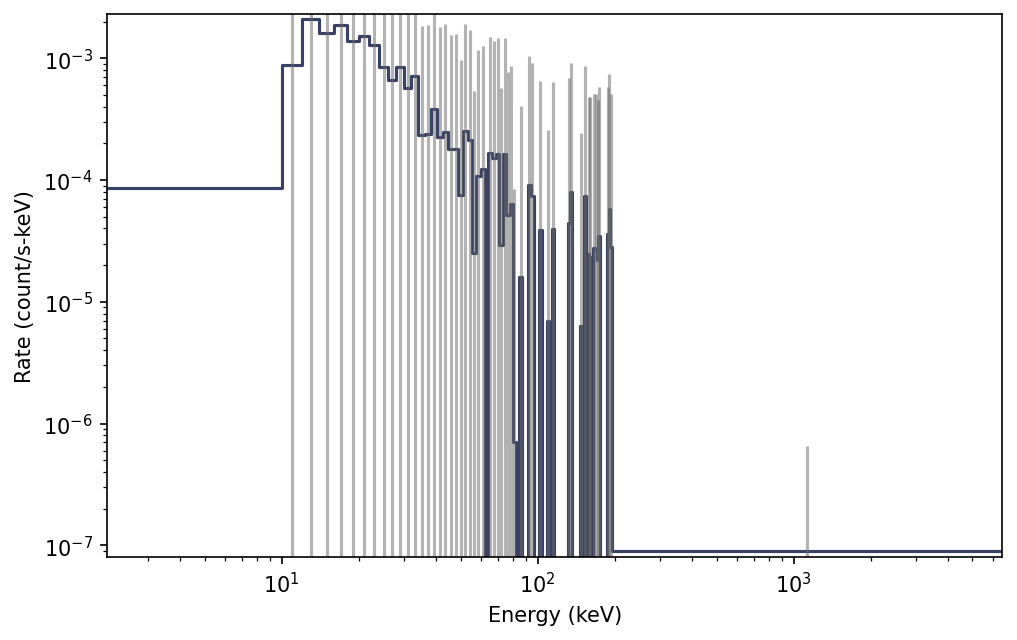
We can plot the energy spectrum:

>>> import matplotlib.pyplot as plt
>>> from gdt.core.plot.spectrum import Spectrum
>>> specplot = Spectrum(data=file.data)
>>> plt.show()

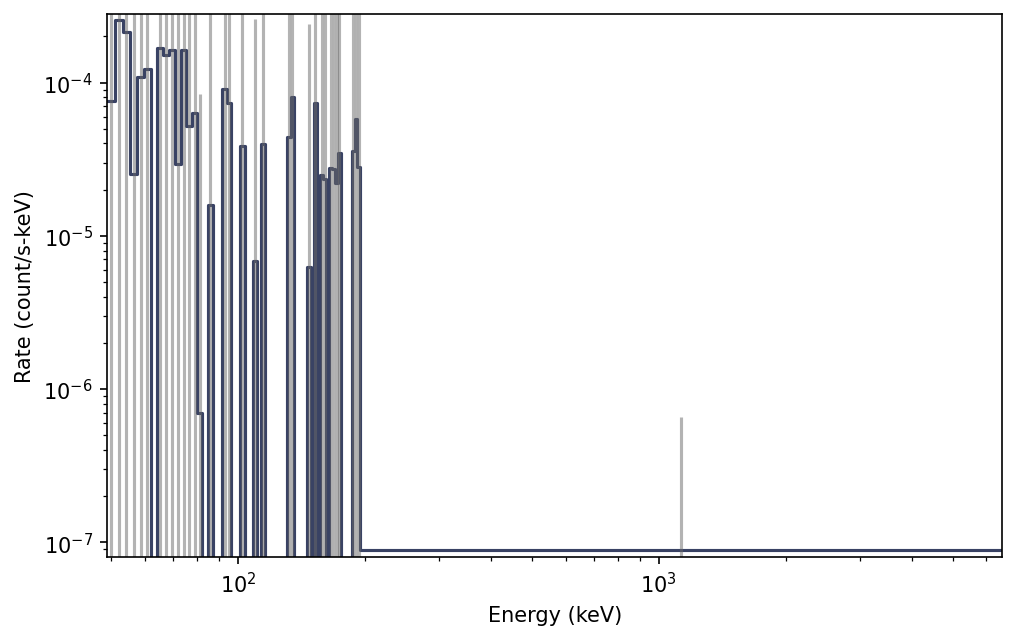
Through the Pha base class, there are a lot of high level functions available to us, such as slicing the data in energy:

>>> energy_sliced = file.slice_energy((50.0, 300.0))
>>> energy_sliced
<BatPha:
  trigger time: 612354468.864;
  time range (69.73658001422882, 113.2039999961853);
  energy range (48.9, 6553.6)>

We can plot the energy-sliced spectrum:

>>> from gdt.core.plot.spectrum import Spectrum
>>> specplot = Spectrum(data=energy_sliced.data)
>>> plt.show()

See Plotting Count Spectra for more on how to modify these plots.

Finally, we can write out a new fully-qualified PHA FITS file after some reduction tasks. For example, we can write out our energy-sliced data object:

>>> energy_sliced_file.write('./', filename='my_first_custom_spectrum.pha')

For more details about working with PHA data, see pha Files.

Reference/API

gdt.missions.swift.bat.pha Module

Classes

BatPha()

Class Inheritance Diagram