Swift BAT Responses (gdt.missions.swift.bat.response)

The BAT response files allow you to compare a theoretical photon spectrum to an observed count spectrum. In short, a single detector response file is only useful for its corresponding detector, for a given source position on the sky, and a given time (or relatively short time span). Essentially, one file contains one or more detector response matrices (DRMs) encoding the energy dispersion and calibration of incoming photons at different energies to recorded energy channels. The matrix also encodes the effective area of the detector as a function of energy for a given source position relative to the detector pointing. This effective area can change dramatically as there is a strong angular-dependence of the response (and the angular-dependence changes with energy!). A file that contains a single DRM will be named with a ‘.rsp’ extension, and a file containing more than one DRM will be named with a ‘.rsp2’ extension. These can be accessed with BatRsp classes, respectively.

Similar to the science data, we can open/read a response file in the following way:

>>> from gdt.core import data_path
>>> from gdt.missions.swift.bat.response import BatRsp
>>> filepath = data_path / 'swift-bat' / 'sw00974827000bevas.rsp.gz'
>>> rsp = BatRsp.open(filepath)
>>> rsp
<BatRsp: sw00974827000bevas.rsp;
trigger time: 612354468.864;
time range (69.73658001422882, 113.2039999961853);
204 energy bins; 80 channels>

There are a number of attributes available to us:

>>> # number of energy channels
>>> rsp.num_chans
80
>>> # number of input photon bins
>>> rsp.num_ebins
204
>>> # time centroids for each DRM
>>> rsp.tcent
91.47029000520706

We can access the DRM directly, which is a ResponseMatrix object:

>>> rsp.drm
<ResponseMatrix: 204 energy bins; 80 channels>

We can fold a photon model through the response matrix to get out a count spectrum. For example, we fold a PowerLaw photon model:

>>> from gdt.core.spectra.functions import PowerLaw
>>> pl = PowerLaw()
>>> # power law with amplitude=0.01, index=-2.0
>>> rsp.fold_spectrum(pl.fit_eval, (0.01, -2.0))
<EnergyBins: 80 bins;
range (0.0, 6553.60009765625);
1 contiguous segments>

This returns an EnergyBins object containing the count spectrum. See Instrument Responses for more information on working with single-DRM responses.

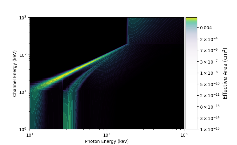
What does a DRM actually look like? We can make a plot of one using the ResponsePlot:

>>> import matplotlib.pyplot as plt
>>> from gdt.core.plot.drm import ResponsePlot
>>> drmplot = ResponsePlot(rsp.drm)
>>> drmplot.xlim = (10.0, 1000.0)
>>> drmplot.ylim = (1.0, 1000.0)
>>> plt.show()

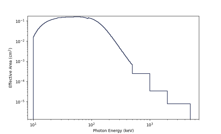
We can also make a plot of the effective area integrated over photon energies using PhotonEffectiveArea:

>>> from gdt.core.plot.drm import PhotonEffectiveArea
>>> effarea_plot = PhotonEffectiveArea(rsp.drm)
effarea_plot.xlim=(8, 7000)
>>> plt.show()

For more details about customizing these plots, see Plotting DRMs and Effective Area.

Reference/API

gdt.missions.swift.bat.response Module

Classes

BatRsp()

Class for BAT single-DRM response files.

Class Inheritance Diagram